The Enumeration and Space-Tiling Motifs of
Marked Polyhedra
by Forrest Bishop January, 2007
© 1994-2007 by Forrest Bishop, All Rights Reserved
Contents
Introduction
Local Orientation Classes (LOCs)
LOC Tiling Motifs of Space
Minimal Kinematically-Compatible Arrays (MKCAs)
Diagonally-marked Cubes and Tilings
Black-and-White Labeled Cubes and Their Tilings
Enumeration of the ‘TS’ Cell Types and MKCAs
Enumeration of the ‘TT’ Cell Types and MKCAs
Glossary
References
Appendix (Images of MKCAs, Cell Type sets, animations)
Introduction
1. Although polyhedra with various markings on them are certainly not unknown, the rigorous enumeration and codification of these kinds of objects does not appear to have been done before, to the best of my knowledge. This electronically-transmitted publication is my first public disclosure, aside from various patents applied for or issued, of apparently previously unknown classes and properties of some of these geometric objects.
2. There are several different ways of distinctively marking the faces of any polyhedron: by labeling with two or more colors, by drawing one or more oriented stripes, with one or more directed stripes, and with combinations of the above. Marking the faces of a cube with undirected lines, or stripes, parallel to the edges of the faces, results in 8 distinct geometric objects. Marking the faces of a cube with undirected lines, or stripes, of two distinct ‘colors’ (‘T’ and ‘S’ or black and white), parallel to the edges of the faces, produces 7 * 32, or 224 distinct geometric objects, while marking the faces with undistinguished, though directed, stripes (‘T’ and ‘T’) results in another 6 * 32, or 192 distinct objects, for a total of 416 different, though related, objects, called individually and collectively Bishop Cubes (R). These objects share various unifying properties partly described by group theory, complexity theory, and space tilings.
3. A most interesting embodiment of these kinds of geometric objects is found in the construction and utilization of a multi-cellular, shape-shifting robot composed of an arbitrary number of similar or identical parts, or cells. The individual cells of this entirely kinetic machine need have no moving parts themselves, as the geometry of the cell’s interface alone suffices to constrain its motion. That application and the already working prototypes of this machine may be described in the companion paper, “‘Bishop Cubes’ (R) and the ‘X Active Cell Aggregate’”.
Local Orientation Classes (LOCs)
4. There exist exactly 8 unique ways to mark a non-oriented cube with stripes such that each of the six faces has only one stripe, placed parallel to an edge of the face. Of these 8 ways, two are mirror images of each other (R-3L and L-3L). These 8 ways are called the (Parallel) Local Orientation Classes (LOCs) (Figure 1.). The designations used in Figure 1. and throughout are based on the visual appearance of each LOC. IOI for example refers to the letters I, O, and then I, which are suggested by the patterns of the stripes.
5. The set {x,y,z} refer to the axes of the global, Cartesian coordinate system, also called the world system. The set {X,Y,Z} refer to the axes of the local Cartesian coordinate system that can be set up on each face of a cube or other parallelepiped. On each such face, ‘X’ and ‘Y’ lie in the plane of the face, with ‘Z’ set as the outward surface normal, often called ‘n’. This convention (small letters for global, capital letters for local) is fairly common in motion control and aerospace. ‘Local’ refers to a particular face of a particular cell, relative to the edges of the face as well as to the other faces.
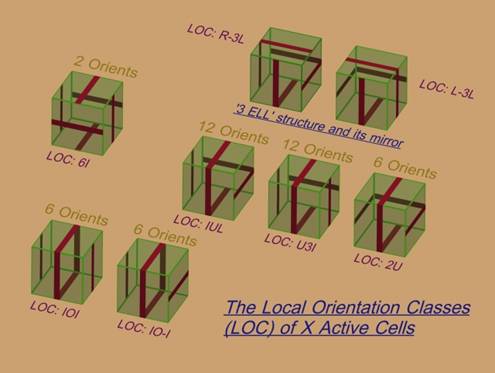
FIGURE 1. The Eight Possible Parallel Local Orientation Classes.
© 2004, Forrest Bishop
6. A proof of the existence of the 8 unique parallel LOCs was constructed by considering all possible ways of marking the faces of oriented cubes with stripes parallel to the edges (Figure 2). For each face there are two possible, mutually-perpendicular stripes. For the six faces there are then 2^6, or 64, possible patterns, without considering the patterns that can be brought into coincidence by rotation or by mirroring.
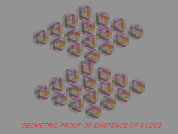
FIGURE 2. Proof of Existence of the Eight Parallel LOCs.
© 2006, Forrest Bishop
7. The number of marked cubes that need to be searched for coincidence can be halved by fixing one face relative to the global coordinates. Figure 2. shows the resulting 32 cubes, with the lower face fixed. The other 32 cubes are generated by rotating the entire array through 90 degrees about the vertical axis, which doesn’t add any new information. The array of 32 cubes was generated by an ordered, binary process of marking each face in one of its two possible orientations. For example, the upper layer is identical to the lower layer, except that the top faces are rotated 90 degrees. A similar arbitrary, though ordered, ‘binary adder’ process was used on the other four faces, obvious by inspection of Figure 2. The colors used on the stripes here are only for reference to the faces.
8. The resulting array of 32 cubes was then searched by inspection to determine which cubes are similar. The 8 LOCs of Figure 1. are the only ones that appear, as labeled in Figure 2. As the array of 32 exhausts all possibilities for marking the cubes by the rules set out in paragraphs 4.-6., this completes the proof.
9. The frequency of appearance appears to give a measure of the complexity, or disorder, of the LOC, with IUL being the most disordered and 6I the most ordered: IUL appears 12 times in the array, and 6I only once. This measure of complexity or disorder loosely governs the sizes of the “Cell Type” sets and arrays (“MKCAs”) described and enumerated below.
10. The spatial relationships between the occurrences of each type of LOC show a variety of interrelationships between them, such as the mirroring of the IO-I and 2U distributions about a vertical, diagonal plane passing through 6I (an almost mirror-symmetry exhibited by the array as a whole), the substitution of 6I at one corner of the lower array for the next-most-ordered IOI appearing at the other three corners, the checkerboard formed by the 3L LOC-types, and its replacement by IUL in the lower array and its displacement of IUL in the upper array. The structure of these relationships is recognizably preserved, though elaborated upon, in the “1024 TT Array” described below.
11. All other 3-space, marked polyhedra can be classified and ordered by a similar method. The markings can be extended to more than two colors, directions, and other such, in an obvious manner. This kind of marking and analysis can be extended to higher-dimension objects in a somewhat less-obvious fashion.
LOC Tiling Motifs of Space
12. Each patterned cube, or LOC, can periodically tile 3-space, trivially as the cube does. To produce a ‘kinematically-compatible’ array, a process of matching oriented markings between two adjacent cubes is carried out for each of the three dimensions of space. Imposing the condition that oriented lines on adjoining faces must match results in an infinite variety of crystal-like structures, or tiling patterns. Imposing the additional restriction that stripes on the other four adjacent faces of each of the two marked cubes must be oriented, in individual pairings, in the same direction also results in an infinity of possible space-tiling patterns. Requiring that the two joined cubes have parallel stripes on their furthest removed parallel faces then reduces the possible space tilings of the LOCs to exactly seven (7) (Figure 3.). These space-tilings, when decorated with sliding interfaces, are called “Minimal Kinematically Compatible Arrays”, or MKCAs. These are the LOC-tilings of greatest interest for the construction of an X Active Cell Aggregate, or a working set of Bishop Cubes(R).
13. An interesting property, that perhaps isn’t immediately obvious, is that mixing members of different LOCs is precluded by the restrictions described in paragraph 12. The kinematically-compatible mixed-LOC arrays cannot result in minimal unit cell-sets smaller than the MKCA of their various member LOCs, though they can produce workable designs of excessive complexity and questionable utility, called “Non-minimal Kinematically Compatible Arrays” (NKCAs). An example from the infinite set of NKCAs is shown in the hyperlinked Appendix.
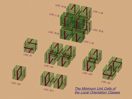
FIGURE 3. ‘Unit Cells’ of the Parallel LOCs.
© 2004-2007, Forrest Bishop
14. For any given LOC, the smallest possible periodic space-tiling unit cell depends on the number of matching pairs of opposite faces of the cube. The eight possible LOCs exhaust all possible cases of 0, 1, 2, or 3 such pairs of matching faces (Figure 3.), also as in Paragraph 18. This minimum-cell-count condition carries through to set the minimum size of the various possible MKCAs of the 224 ‘TS’ and the 192 ‘TT’ cells described below. An elaboration of the face-matching condition also sets the number of these possible space-tiling motifs to four, as described below.
15. A second measure of complexity or disorder is seen in the number of fundamental LOC cells needed to form the ‘unit cell’ of a LOC array. 6I and IOI only need a single cell to tile space, while IUL needs four such cells in four different orientations. R-3L and L-3L have to join up, with four of each type appearing in different orientations to produce an 8-member ‘unit cell’. The movement of this type of MKCA is different from, e.g. 6I, in that subsets of the 8-member 3L array can be moved independently, but then have to be brought back into a rest configuration in order to make an orthogonal move.
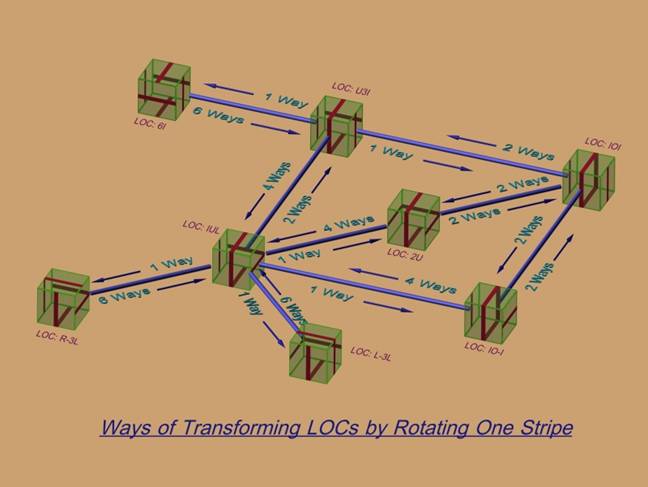
FIGURE 4. Transforming Between the Parallel LOCs.
© 2004- 2007, Forrest Bishop
16. The 8 LOCs above form a group of sorts under the transformation rule: “one stripe is rotated about local ‘Z’ axis”. As shown in Figure 4., there are six ‘ways” out of each node, or LOC, which correspond to rotating one of the six stripes on one of the six faces. There are then 48 total ways to transform from one LOC to another. 24 of these ways transform into IUL, 10 into U3I, 5 into IOI, 3 into IO-I, and one way each into 6I, R-3L, and L-3L. By these statistics, IUL is as likely to form in a random process as all the rest of the LOCs combined. The discrepancy between this 0.5 probability and the 0.375 probability of Paragraph 9. is due to the path-dependency of the transform.
Minimal Kinematically-Compatible Arrays (MKCA)
17. The Cell-Types within each Local Orientation Class (LOC) fall into four fundamental patterns of space-tilings, regardless of whether the faces are labeled with two colors, or marked as ‘TS’ or as ‘TT’ (described below), and regardless of LOC-type. These four infinite tiling patterns share the property of infinite planes which contain face-markings all oriented in the same direction. An embodiment of that property, with the markings being the directions of sliding freedom for the cells, results in a crystal-like substance that can be divided, such that two adjoining sections of it are capable of moving relative to each other, along the axes of the markings, and then serially in the three dimensions. The arrays of cells thus formed are therefore called Minimal Kinematically-Compatible Arrays (MKCAs).
18. These four fundamental, labeled or marked-parallelepipedal space-tiling matching-conditions are named:
a) 3M, for “three pairs of matching, opposed faces”
b) 2M, for “two pairs of matching, opposed faces”
c) 1M, for “one pair of matching, opposed faces”
d) 0M, for “no matching, opposed faces”
The ‘unit cells’ in Figure 3. show each of these types of tilings, as described in Paragraphs 12-14. A tiling is so named if at least one of its Members (and therefore all of them by the Genetrix Property described in Paragraph 20.) has the matching (or ‘anti-matching’) condition. These four matching-conditions result in four distinguishable motifs or three-dimensional tiling patterns. These motifs are named:
a) for 3M: “Adjacent 3 x 3”, or “Whorl”
b) for 2M: “Adjacent 2 x 4”
c) for 1M: “Baseball”
d) for 0M, “Jigsaw”
19. Figures 6. and 8. for example show these space-tiling motifs. The Adjacent 3x3, or Whorl, MKCA may contain 1, 2, 4, or 8 cells, depending on the properties of the particular LOC as well as the markings. The Adjacent 2x4 MKCA may contain 2, 4, or 8 Members, depending on the properties of the particular LOC. The Baseball MKCA may contain 4 or 8 Members, and the Jigsaw MKCA is always composed of 8 Members, which may or may not be unique. Each motif has a more nuanced structure than the matching-face condition alone implies, hence the additional nomenclature, intended to evoke some of these recurring, three-dimensional features. Figure 8. below shows the simplest possible realization of these four structures, as “one of two possible colors per face” is less information than “one of two possible local orientations per face”.
20. MKCA Genetrix Property:
Any Member of a MKCA can generate all the other Members (i.e. Cell Types, repeated or otherwise) of the same MKCA.
The generation of the other Members of a particular MKCA follow the rules set out in e.g. Paragraph 12., with the additional constraint of similar face-types. Thus, any Member can be considered the Genetrix of the MKCA. There may only be 8, 4, 2, or 1 Cell Types in a Minimal Kinematically-Compatible Array. Because of the Genetrix Property,
a Cell Type that is a Member of one kind of MKCA cannot also be a Member of a different kind of MKCA.
This Exclusion Property, taken together with the Four-Motifs property of Paragraph 18., also provides a cross-check on the number of distinct, marked cubes.
Diagonally-marked Cubes and Tilings
21. For another example of a finite set of marked polyhedra, the marking rule of Paragraph 4. is replaced with “mark a non-oriented cube with stripes such that each of the six faces has only one stripe, placed diagonally on the face”. There exist eight (8) unique ways to do this, depicted in Figure 5., one of which is the well-known inscribed tetrahedron. The structure of this set shares some other similarities with the parallel LOCs described above.
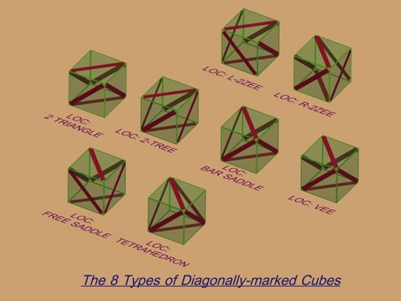
FIGURE 5. The Set of Eight Possible Types of Diagonally-marked Cubes.
© 2004-2007, Forrest Bishop
22. Each diagonally-striped cube, or diagonal-LOC, can regularly tile 3-space, trivially as the cube does. To produce a ‘kinematically-compatible’ array, a process of matching oriented markings between two adjacent cubes is carried out for each of the three dimensions of space. Imposing the condition, as in Paragraph 12., that oriented lines on adjoining faces must match results in an infinite variety of crystal-like structures, or tiling patterns. Imposing the additional restriction that stripes on the other four adjacent faces of each of the two marked cubes must be oriented, in individual pairings, in the same direction also results in an infinity of possible space-tiling patterns. Requiring that the two joined cubes have parallel stripes on their furthest removed parallel faces then reduces the possible space tilings of the Diagonal LOCs to exactly five (5) (Figure 6.).
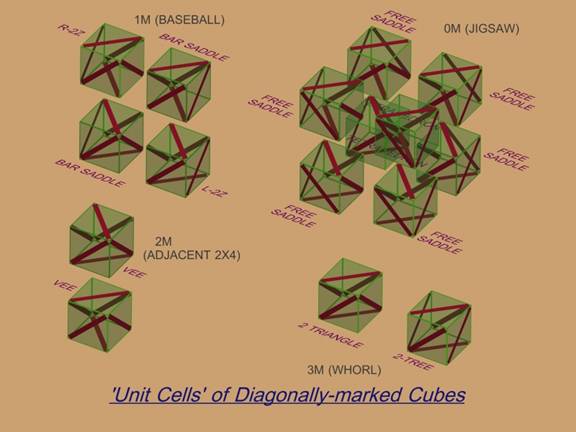
FIGURE 6. The Set of Five Possible ‘Unit Cells’ of the Diagonally-marked Cubes. © 2007, Forrest Bishop
23. The two types of the “3 matching pairs of opposing faces’,“3M”, or “Adjacent 3 x 3”, or “Whorl” tiling suggest why those names were chosen. “Baseball” is less clear- it is the ‘2Z’ cells which correspond to, and map onto the positions and orientations of, the ‘3TO’s of Figure 8. below, with ‘Bar Saddle’ corresponding to ‘1T’ and ‘5T’. The two V-shapes formed within the ‘Vee’ type correspond and map to the adjacent two colored faces in “Adjacent 2 x 4” of Figure 8.The two “Tetrahedrons” in “Jigsaw” map onto the ‘0T’ and ‘6T’ cells of Figure 8., with the ‘Free Saddle’ types corresponding to the ‘2TO’ and 4TO’. For these diagonally-marked cubes, the different LOCs sometimes have to be mixed together to form the space tilings, different from the assertion in Paragraph 13.
Black-and-White Labeled Cubes and Their Tilings
24. Two colors, labeling the faces of cubes, produce ten (10) unique types. These are a previously-known set, corresponding to a magnetic color group. The convention used in Figure 7. replaces the two colors with large and small circles, simply for ease of visualization. The distinguishable orientations are also labeled. ‘3TO’ means “three faces labeled say white (or ‘T’), two of which are on opposite sides of the cube. ‘3TA’ is “three labeled faces Adjacent”, and so on. Below, ‘T” and ’S’ are used instead of “White” and “Black”.
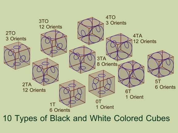
FIGURE 7. The Ten Ways to Label a Cube’s Faces with Two Colors
© 2004-2007, Forrest Bishop
25. The ten “Black and White” cell types form and originate the four space tiling ‘unit cells’ as above. As fifteen cells are required, some of the cell types have to appear more than once, though in different orientations- a typical result for all the tilings. It is the frequency, positions, and orientations within the ‘unit cells’ that allow comparison between very differently labeled or marked polyhedra, as referred to in Paragraph 23.
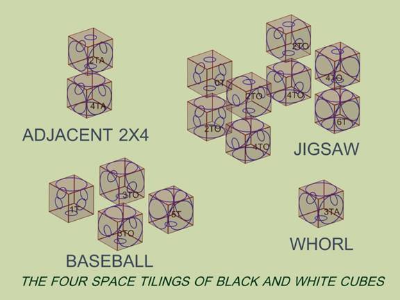
FIGURE 8. The Set of Four Possible ‘Unit Cells’ of Two-Color Cubes.
© 2007, Forrest Bishop
Enumeration of the TS Cell Types and MKCAs
26. There are two ways of marking non-colored, parallel stripes on a cube, described in Paragraph 2, either directed or not. The non-directed, parallel-striped Cell Types which are additionally marked with two colors are called “TS Cells”. There appear to be 7 * 32, or 224, unique types of TS Cells, divided among the eight parallel LOCs, as shown in Table 1, where “TS Type” uses the nomenclature of Figure 7. All of these Cell Types, and their associated, space-tiling MKCAs, should be depicted in the hyperlinked images found in the Appendix below.
The Set of All Possible Cell Types Composed of ‘T’ and ‘S’ Faces |
|||||||||
|
TS Type |
Parallel Local Orientation Class (LOC) |
Totals |
|||||||
|
|
6I |
IOI |
R-3L |
L-3L |
U3I |
2U |
IO-I |
IUL |
|
|
0T |
1 |
1 |
1 |
1 |
1 |
1 |
1 |
1 |
8 |
|
1T |
1 |
3 |
1 |
1 |
4 |
2 |
2 |
6 |
20 |
|
2TA |
1 |
3 |
3 |
3 |
6 |
4 |
4 |
12 |
36 |
|
2TO |
1 |
3 |
1 |
1 |
3 |
2 |
2 |
3 |
16 |
|
3TA |
2 |
2 |
2 |
2 |
4 |
2 |
2 |
8 |
24 |
|
3TO |
2 |
6 |
2 |
2 |
8 |
4 |
4 |
12 |
40 |
|
4TA |
1 |
3 |
3 |
3 |
6 |
4 |
4 |
12 |
36 |
|
4TO |
1 |
3 |
1 |
1 |
3 |
2 |
2 |
3 |
16 |
|
5T |
1 |
3 |
1 |
1 |
4 |
2 |
2 |
6 |
20 |
|
6T |
1 |
1 |
1 |
1 |
1 |
1 |
1 |
1 |
8 |
|
Totals: |
12 |
28 |
16 |
16 |
40 |
24 |
24 |
64 |
224 |
TABLE 1. The 224 Possible ‘TS’ Cell Types.
© 2004-2007, Forrest Bishop
27. For the eight possible non- rotating LOCs, there are 8 * 64 = 512 possible, distinct TS cells. This can be seen by imagining the cube marked with the pattern of a LOC held stationary as all 64 B&W patterns are tried out on it. The duplicates are then found by rotating them into coincidence with one another, which only can be done for the coincident orientations of the LOC itself. The mirror images are considered to be separate objects.
|
Number and Types of ‘TS’ MKCAs in Each Parallel LOC |
|||||||||
|
MKCA Motif |
# of Cells in MKCA |
Frequency of Appearance of MKCA in the Local Orientation Class (LOC) |
|||||||
|
|
|
6I |
IOI |
R-3L |
L-3L |
U3I |
2U |
IO-I |
IUL |
|
Whorl (1) |
1 |
2 |
2 |
0 |
0 |
0 |
0 |
0 |
|
|
Whorl (2) |
2 |
0 |
0 |
0 |
2 |
1 |
1 |
0 |
|
|
Whorl (4) |
4 |
0 |
0 |
0 |
0 |
0 |
0 |
2 |
|
|
Whorl (8) |
8 |
0 |
0 |
1 |
0 |
0 |
0 |
0 |
|
|
|
|
|
|
|
|
|
|
|
|
|
Adjacent 2x4 (2) |
2 |
1 |
3 |
0 |
2 |
2 |
2 |
0 |
|
|
Adjacent 2x4 (4) |
4 |
0 |
0 |
0 |
2 |
1 |
1 |
4 |
|
|
Adjacent 2x4 (8) |
8 |
0 |
0 |
1 |
0 |
0 |
0 |
1 |
|
|
|
|
|
|
|
|
|
|
|
|
|
Baseball (4) |
4 |
1 |
3 |
0 |
2 |
2 |
1 |
2 |
|
|
Baseball (8) |
8 |
0 |
0 |
1 |
1 |
0 |
2 |
2 |
|
|
|
|
|
|
|
|
|
|
|
|
|
Jigsaw |
8 |
1 |
1 |
2 |
1 |
1 |
1 |
1 |
|
|
|
|
|
|
|
|
|
|
|
|
|
Total # of ‘TS’ MKCAs in LOC |
|
5 |
9 |
5 |
10 |
7 |
8 |
12 |
|
TABLE 2. The MKCAs of the ‘TS’ Cell Types.
© 2004-2007, Forrest Bishop
28. Each set of unique ‘TS’ Cell Types of a particular LOC tiles space in each of the four possible ways described in Paragraph 18. The number of Members in each MKCA varies- IUL has the richest set, and 6I the simplest. The 3L MKCAs are all composed of R-3L intermixed with L-3L in an eight-celled 3D checkerboard, just as in Figure 3, and regardless of motif. The total number of possible ‘TS’ MKCA-type space-tilings spanning all 8 parallel LOCs is 7 * 8 = 56, which is exactly one-fourth the number of ‘TS’ Cell Types. I conjecture that these (Table 2.) are also the partial and total numbers and kinds of ‘TT’ MKCAs, though this has not been rigorously checked. Then Table 4. below will be identical to Table 2.
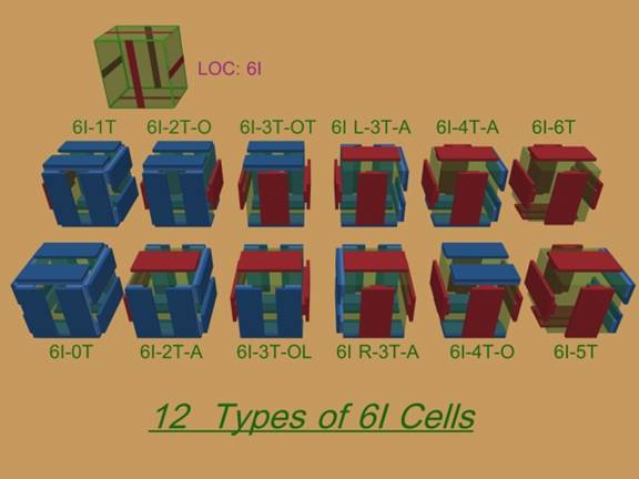
FIGURE 9. The Set of Twelve Possible Types of 6I-TS Cells.
© 2004-2007, Forrest Bishop
29. Figure 9. shows the 12 unique “6I-TS Cell Types, with an earlier version of the nomenclature used to individually identify each Cell Type. No Cell Type can be rotated into coincidence with another. Mirror-images are considered to be unique. The “6I L-3T-A” is a mirror of the “6I R-3T-A”. Figure 10. shows the five 6I-TS MKCAs called out in Table 2. Each uses the smallest possible ‘unit cell’ of its motif. “KCS” means MKCA. The two colors, red and blue, are elaborated into the sliding interfaces of a cellular robot.
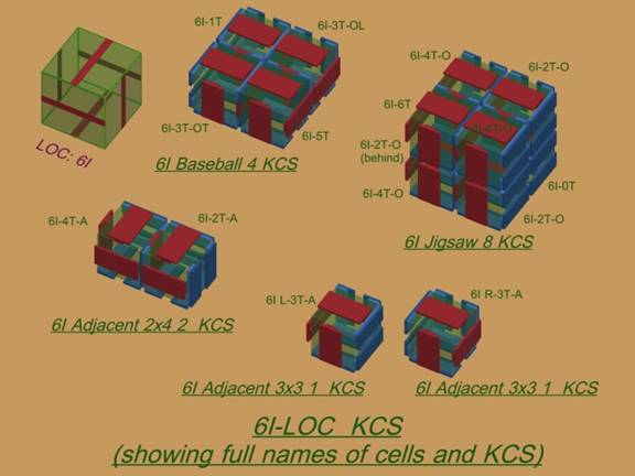
FIGURE 10. The Set of Five Possible Types of 6I-TS MKCAs.
© 2004-2007, Forrest Bishop
Enumeration of the TT Cell Types and MKCAs
30. A problem arises when attempting to enumerate these objects by construction. For the TS Cell Type the faces have bilateral symmetry, so mirroring a face does not change its aspects, nor its relations to the other faces. For the TT cell type, the asymmetry of the directed arrow introduces a new element in the three-dimensional relationships between the six faces of the decorated cube. Mirroring a single face therefore changes the Cell Type. This cannot be discovered by mirroring the cells themselves, and possibly not by a group-theoretic approach either. The resulting sets of Cell Types may or may not be isomorphic to any known group.
31. There are just four ways to orient a directed line, or arrow, parallel to an edge of a non-rotating square. The arrow can be replaced with an equivalent, marked edge of the square. In either case, for the six faces involved, there are then 4^6, or 4096 different ways to place directed lines on a non-rotating cube. Many of these are reoriented copies of the same pattern. We are interested in the finite set of unique Cell Types. One process of elimination of duplicates is to map onto the 8, non-rotating, LOC members, which restricts the direction of the arrow to two choices. Then there is a ceiling of 2^6 = 64 possibilities for each type of LOC, for a total of 8 * 64 = 512 possibilities. The problem of counting all the distinct TT X Cell Types then reduces to eliminating the rotationally-equivalent cases.
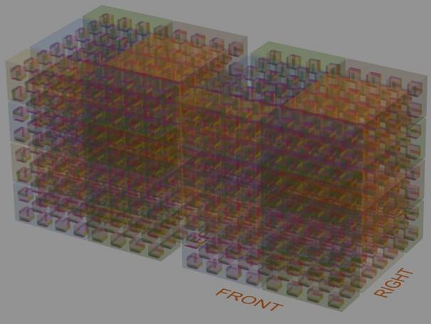
FIGURE 11. An Array of 1024 TT Cell Types. © 2006, Forrest Bishop
32. A more interesting method of sifting out the distinct members is to form an array of all 4096 possibilities by following rules of construction similar to those described in Paragraph 6., and shown in Figure 2. These 4096 cases can be reduced to 1024 by fixing one of the local marking orientations (e.g. the mark on the bottom face), on one of the faces, in global space (Figure 11). Then the other 3072 cases are found by simply rotating the entire array through three increments of 90 degrees each, about the vertical axis. The array is further split into two blocks of 512 non-unique Cell Types each, similar to Figure 2., by rotating the top marks through 90 degrees. These two side-by-side blocks in Figures 11. and 12. correspond to the two layers depicted in Figure 2. “512P” refers to the top and bottom marks being parallel, while “512X” refers to these marks being mutually orthogonal.
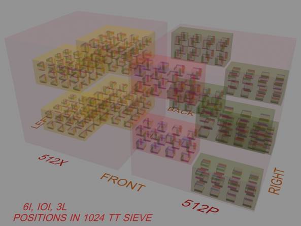
FIGURE 12. Positions and Frequencies of Some of the LOC-Members in the 1024 TT Array. © 2007, Forrest Bishop
33. By this method, the information pertaining to the relationships between the various sets of LOC-constrained Cell Types is preserved, which would be lost by the parsing described in Paragraph 30. These are shown as colored, transparent blocks, which form a structure within the 1024 TT Array, closely related to the structure described in Paragraph 10. For example, L-3L and R-3L, shown inside yellow boxes, can only appear in the 512X block, where they form a 3D checkerboard similar to the 2D layout in Figure 2. 6I (red boxes) and IOI (green boxes) can only appear in the 512P block. This kind of search by construction can be extended to any form of marked polyhedra of any dimension.
34.
The Set of All Possible Cell Types Composed of ‘T’ and ‘T’ Faces |
|||||||||
|
TT Cell Type |
Parallel Local Orientation Class (LOC) |
Totals |
|||||||
|
|
6I |
IOI |
R-3L |
L-3L |
U3I |
2U |
IO-I |
IUL |
|
|
Totals: |
8 |
18 |
16 |
16 |
32 |
20 |
20 |
64 |
192 |
TABLE 3. The 192 TT Cell Types.
© 2004-2007, Forrest Bishop
|
Number and Types of ‘TT’ MKCAs in Each Parallel LOC |
|||||||||
|
MKCA Motif |
# of Cells in MKCA |
Frequency of Appearance of MKCA in the Local Orientation Class (LOC) |
|||||||
|
|
|
6I |
IOI |
R-3L |
L-3L |
U3I |
2U |
IO-I |
IUL |
|
Whorl (1) |
1 |
2 |
2 |
0 |
|
|
|
|
|
|
Whorl (2) |
2 |
0 |
0 |
0 |
|
|
|
|
|
|
Whorl (4) |
4 |
0 |
0 |
0 |
|
|
|
|
|
|
Whorl (8) |
8 |
0 |
0 |
1 |
|
|
|
|
|
|
|
|
|
|
|
|
|
|
|
|
|
Adjacent 2x4 (2) |
2 |
1 |
3 |
0 |
|
|
|
|
|
|
Adjacent 2x4 (4) |
4 |
0 |
0 |
0 |
|
|
|
|
|
|
Adjacent 2x4 (8) |
8 |
0 |
0 |
1 |
|
|
|
|
|
|
|
|
|
|
|
|
|
|
|
|
|
Baseball (4) |
4 |
1 |
3 |
0 |
|
|
|
|
|
|
Baseball (8) |
8 |
0 |
0 |
1 |
|
|
|
|
|
|
|
|
|
|
|
|
|
|
|
|
|
Jigsaw |
8 |
1 |
1 |
2 |
|
|
|
|
|
|
|
|
|
|
|
|
|
|
|
|
|
Total # of ‘TT’ MKCAs in LOC |
|
5 |
9 |
5 |
? |
? |
? |
? |
|
TABLE 4. Some of the MKCAs of the ‘TT’ Cell Types.
© 2004-2007, Forrest Bishop
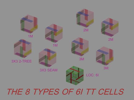
FIGURE 13. The Set of Eight Types of 6I-TT Cells, Sifted Out from the 1024 TT Array.
© 2006, Forrest Bishop
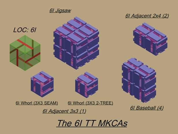
FIGURE 14. The Five Possible 6I-TT MKCAs.
© 2004-2007, Forrest Bishop
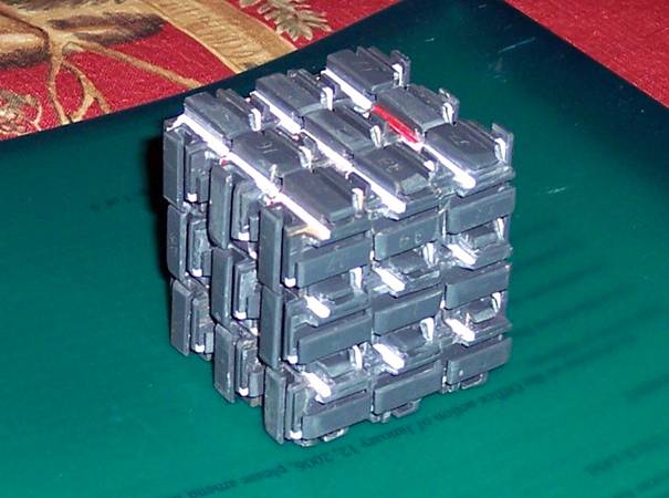
FIGURE 15. The Original Working Prototype.
Out of the 416 possible kinds of parallel-LOC Bishop Cubes™, “6I-TT 3x3 SEAM” was selected for the Cell Type and MKCA of the twenty-seven identical Cells of the original working prototype.
Glossary
Some of these terms are from my 1995 paper “The Construction and Utilization of Space Filling Polyhedra for Active Mesostructures”, at www.iase.cc
[A], etc.: A specific configuration of a given aggregate.
[A]->[B]: Change the shape of an Aggregate from configuration [A] to configuration [B].
Active Cell: A standardized machine, capable of interfacing and interacting with identical units.
Aggregate: A number of standard cells connected together by their mutual interfaces.
(ACA) Active Cell Aggregate: a connected collection of Active Cells.
Cell: a) The smallest complete unit of a Cellular Automata, or of a Kinematic Cellular Automata, or of an Active Cell Aggregate.
Cell Metric: a) The nominal lengths, edge angles, and face angles of the smallest cell (the Unit Cell) of a particular system. b) The nominal edge length of a cell. c) The distance between centroids of adjacent cells.
Cell Type: The unique geometric properties of a Cell, including polyhedron type, local orientation of degrees of freedom, markings and labels, and interface type.
Composite Cell: A group of cells that form a larger cell similar to the cell metric.
Configuration: An arrangement of the cells in an aggregate in which all cells are centered and aligned at the cell metric.
Configuration Space: All of the possible configurations of an aggregate. Motion primitives form the links between configurations. There are three types of mutually exclusive spaces comprising one, two, and three dimensioned aggregates.
Faceplate: The physical implementation of a geometric face of a polyhedron.
Figure Game: A permitted trajectory in configuration space, from one configuration to another. A set of linked motion primitives between two arbitrary configurations.
[A]->[B] Figure Game Set: For any two configurations, the set of all possible trajectories between them.
Fully Packed: No internal voids in the Aggregate- all cell positions occupied.
Group: A subset of an aggregate.
Kinematically-Compatible Array (KCA): An Active Cell Aggregate composed of Cells able to move in groups with respect to other groups.
Minimal Kinematically-Compatible Array (MKCA): The smallest number of Cells required for full motion along all possible degrees of freedom.
Mode of Motion, Motion Macro: A method of moving a group or groups of cells in an aggregate.
Rest Position: An inactive configuration of an Active Cell Aggregate, consisting of two or more connected Active Cells, with their respective faces coplanar.
Standard Interface, Standard Face: The mechanical, power, and signal interfaces on a particular faceplate of a standardized Active Cell.
Terminus: A configuration that an Aggregate, or part of an Aggregate, has to assume (by necessity or by design) at some point in a Figure Game.
Unit Cell: The smallest number of Active Cells that form a Kinematically Compatible Array.
X Active Cell: A Cell capable of motion only in local ‘X’ or only in local ‘Y’ axes, but not in local ‘Z’.
XY Active Cell: A Cell capable of motion in local ‘X’ or in local ‘Y’ axes, but not in local ‘Z’.
XZ Active Cell: A Cell capable of motion only in local ‘X’ or only in local ‘Y’ axes, and also able to disconnect in local ‘Z’.
XYZ Active Cell: A KCA Cell capable of motion in local ‘X’ or in local ‘Y’ axes, or in local ‘Z’.
References, Errata, Notes
“The Construction and Utilization of Space Filling Polyhedra for Active Mesostructures”, at www.iase.cc
“Space-filling polyhedra” is not a correct terminology, as there exist such without sliding planes, e.g.: Interlocking Toroidal Tile for Tessellating R3
by Carlo H. Séquin
http://http.cs.berkeley.edu/~sequin/GEOM/looptile.html
Wang Tiles, Wang Cubes
Appendix
Hyperlinks to Images of all MKCAs, Cell Type Sets, and Animations. Not completed in this draft.